Overview

This course will introduce you basic concepts in Artificial Intelligence including the following:

• Search algorithms: Global and Local
• A bit of game theory: Minimax with Alpha-Beta pruning
• How to solve Constraint Satisfaction Problem (CSP) such as job scheduling
• Logic: Propositional Logic and First Order Logic (make sure not to confuse between these two)
• Machine Learning: ID3 Tree
• Deep Learning: Perceptron, Multi Layer Perceptron and Backpropagation

Do not be overwhelmed by this. After you read this blog, you will understand it easier. I can not guarantee you will understand all of those concepts after reading this blog. But I can guarantee you will not make the same mistake that I did.

Search algorithms

Do you know Depth-First Search, Breadth-First Search and Dijkstra? You may learn it in DSA course, and yes, Global Search is about those (and a bit more). If you are not familiar with those, you can find many visualization and tutorial on the internet about DFS, BFS and Dijkstra.

Global Search

Global Search algorithms are split to Uninformed search, which consists DFS, BFS and Uniform Cost Search (UCS, aka Dijkstra in disguise), and Informed search, which consists Greedy BFS (GBFS), A* algorithm. Uninformed search algorithm "is given no clue about how close a state is to the goal(s)" while Informed search is. Optional reading will covers Depth-limited search (DLS) and Iterative deepening search (IDS), which are variants of DFS, for uninformed search and Weighted A*, Memory bounded search for informed search. In global search, you should focus about the definition of a "node" (vs a "value"), "frontier", a node being "expanded", "graph search" vs "tree search", and "early-goal" vs "late-goal" test.

• "Frontier" is a data structure to store the "node", which consists values. Frontier is a stack in DFS, a queue in BFS and a priority queue in UCS, GBFS and A*.
• "Graph search" checks redundant paths (cycle and loopy paths) while "Tree search" does not.
• "Early-goal" test is when the algorithm halts after generating the goal, while "Late-goal" test halts only when the goal is "expanded", which is being popped from the "frontier". Early-goal are often use in DFS, BFS, GBFS and late-goal for others.

In A*, two importants concepts you should remember are Admissibility and Consistency:

Admissible heuristic is when the heuristic never larger than the true cost from that node to the goal. Admissibility allows the heuristic to find the optimal cost.

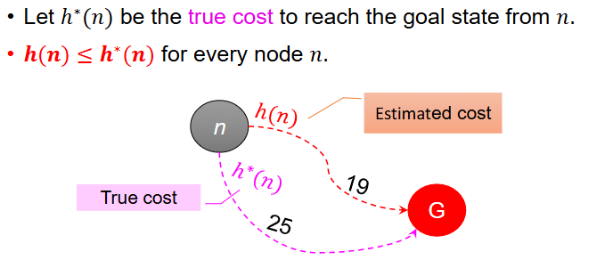
Figure: Admissible heuristic where estimated cost never exceeds true cost to the goal.

Consistent heuristic is when the moment we expand a node, it is the optimal path to that node. Consistency allows the heuristic to not visit a node twice. Note that Every consistent heuristic is admissible (but not vice versa).

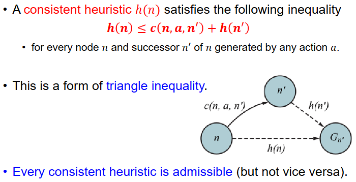
Figure: Consistent heuristic satisfying the triangle inequality condition.

Local search

You will learn four common algorithms: Hill climbing, Simulated Annealing, Local Beam search and Evolutionary algorithms. Hill climbing has variants such as Stochastic hill climbing, First-choice hill climbing and Random-restart hill climbing in order to avoid end up at local maxima, ridges (a sequence of local maxima, better than surrounding landscape but global maxima direction is not aligned with agent's available actions) and plateaus (flat area in state-space landscape). Local Beam search iteratively search k path -> choose top k path -> repeat.

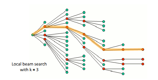
Figure: Local beam search keeps the best k=3 candidates at each iteration.

Evolutionary algorithms consists 3 stage: selection, recombination, and mutation then repeat. Selection process uses fitness function (measure how good the current individual is) and roulette method to decide (fitness function higher -> higher chance of being choose from). Recombination happens at crossover points where parents interchange their parts. Mutation is when the model will randomly perturb the offspring's bit to simulate mutation in real world. Evolutionary algorithms have many advantages such as it relies on very little domain knowledge or it haves large number of “tunable” parameters but it lacks of good empirical studies comparing to simpler methods.

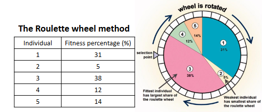
Figure: Roulette-wheel selection gives higher-fitness individuals higher sampling probability.

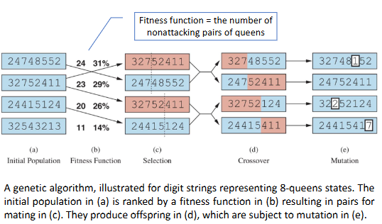
Figure: Evolutionary algorithm loop with selection, crossover, and mutation.

Minimax and Alpha-beta pruning

Minimax relate to game theory where two players try to pick actions that maximize/minimize other's score. The algorithm is simple: at MAX nodes, you choose the maximum value of all children and do the opposite for MIN nodes. Alpha-beta pruning's intuition lies in the fact that we can skip some nodes or subtree and still get the same result as minimax. Alpha-beta pruning introduce $\alpha$ and $\beta$ which are minimum and maximum value we can get at the current node, respectively. You will learn more in the course but you can simply remember this: "MAX node updated left/alpha ($\alpha$ get updated after traversing one of its subtrees) and MIN node updated right/beta ($\beta$ get updated after traversing one of its subtrees). We prune all remaining subtrees of this node when $\alpha$ and $\beta$ range is invalid, which is $\alpha \ge \beta$ (remember the inclusion of = sign)".

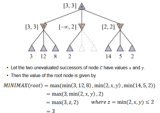
Figure: Alpha-beta pruning skips branches that cannot affect the final minimax decision.

Constraint Satisfaction Problems (CSPs)

These are problems where you have variables that need to assign some value in its domain (allowed value). You will learn "unary/binary constraint" (depend on the number of variables in the constraint), "forward checking" to remove domain value that conflict with existing constraints and "AC-3" (forward checking but can propagate). To solve CSP, we can formulate it as a search problem and use backtracking with some heuristic such as Minimum Remaining Value (MRV), Degree Heuristic (DH) and Least Constraining Value (LCV) to choose which variables and which values to fill.

Logic

This is a hard section, so I will try to summarize it. But the core of this section is check whether KB entails $\alpha$ or in other words, check whether we can prove that a new logic is wrong (or conflict) compared to current set of logic! Important concept: concept of "satisfiable", resolution refutation, "substitute", "skolemize" and forward/backward chaining algorithms.

Propositional Logic (PL)

First thing we should know is a property of Knowledge-based (KB) agents: "Knowledge-based agents perform reasoning over an internal representation of knowledge to decide what actions to take". KB agents involves a Knowledge base (KB), a set of sentences or facts, and Inference, which is a process where agents derive new sentences from old ones. A simple inference procedure tries to check whether KB entail ($\models$) a sentence $\alpha$ or not. But what is entailment? "Entailment is a relationship between sentences (i.e., syntax) that is based on semantics" and $\alpha$ entails $\beta$ if and only if, in every model which $\alpha$ is true, $\beta$ is also true.

The syntax in PL can be summarized as this:

• Sentence is either Atomic Sentence or Complex Sentence
• Atomic Sentence is simple True, False or P, Q, R,...
• Complex Sentence is a Sentence, negation of a Sentence or multiple Sentences connected using operators
• Operator precedence: $\neg$, $\land$, $\lor$, $\implies$, $\iff$
• CNF Sentence is $Clause_1 \land \dots \land Clause_n$
• Clause is $Literal_1 \lor \dots \lor Literal_m$
• Literal is Symbol or negation of Symbol
• Symbol is the letter P, Q, R,...
• Horn Clause form is either Definite Clause form or Goal Clause form
• Definite Clause form is $Symbol_1 \land \dots \land Symbol_n \implies Symbol$ (Every definite clause can be written as an implication)
• Goal Clause form is $Symbol_1 \land \dots \land Symbol_n \implies False$

We also have concept of "validity" and "satisfiability".

• A sentence is valid if it is true in all models.
• A sentence is satisfiable if it is true in some models.
• A sentence is unsatisfiable if it is true in no models. Ideally, you can use either Proof by refutation or Proof by contradiction to see if $\alpha \models \beta$.

To answer the question "Does KB semantically entail $\alpha$?", we can use Model-checking approach, Inference rules or Resolution refutation (inverse SAT problem, where we will prove that opposite of $\alpha$ conflicts the facts in KB and thus KB should entail $\alpha$).

• Model-checking approach: write Truth table and see if $\alpha$ is true in every model where KB is true => sound and complete.
• Inference rules: apply inference rules directly to sentences in KB. Some sound rules such as Modus Ponens, Modus Tollens, AND-Introduction and AND-Elimination.
• Resolution refutation: "resolution is a single inference rule that yields a complete inference algorithm when coupled with any complete search algorithm". It consists Unit resolution inference rule (or more general, Full resolution rule). Resolution applies only to clauses so we need to convert all sentences to Conjunctive Normal Form (CNF) by eliminate $\iff$, $\implies$ and then move negation and apply distributivity law to distribute $\lor$ over $\land$. After that, we prove $KB \models \alpha$ by showing that $KB \land \neg \alpha$ is unsatisfiable.

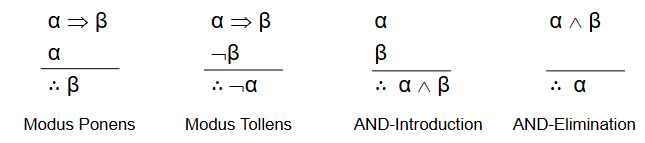
Figure: Modus ponens and related inference rules used in propositional reasoning.

When KB only contains definite clauses, we can use forward chaining and backward chaining to do the inference:

• Forward chaining: Fire any rule whose premises are satisfied in the KB, add its conclusion to the KB, until the query is found. The algorithm is data-driven, automatic, unconscious processing.
• Backward chaining: Work backwards from the query. The algorithm is goal-driven, good for problem-solving.

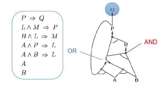
Figure: Forward chaining expands known facts until the target query Q is derived.

First-Order Logic (FOL)

In propositional logic, knowledge and inference are separate, with inference being domain-independent. The syntax and semantics of first-order logic is built around objects and relations. FOL concepts involves symbols: constant symbol represents object, predicate symbol represents relation and function symbol represents functions.

FOL syntax is more diverse than PL with quantifier and term:

• Quantifier is $\forall$ and $\exist$.
• Constant: A, X1, John,... (the first letter is uppercase)
• Variable: a, x, s,... => A variable may serve as the argument of a function.
• Predicate: True, False, Loves, After, Running,...
• Term is Function of Terms or a constant or a variable. Term is a logical expression that refers to an object. A term with no variable is called a ground term.
• Atomic sentence is now a predicate of terms (e.g. Brother(Richard, John), Married(Father(Richard), Mother(John)))

Quantifiers:

• Typically, $\implies$ is the main connective with $\forall$, do not use $\land$ because it impose too strong implication. For example: $\forall x, Student(x, FIT) \land Smart(x)$ means "Everyone is a FIT student and Everyone is smart." rather than "Everyone FIT students is smart".
• And $\exist$ has $\land$ as the main connective instead of $\implies$ because $\implies$ impose week implication.
• The order of quantification is therefore very important. Quantifiers are related to each other via negation (use De Morgan's rule)

There is $=$ sign but not $\ne$, instead we use $\neg (x = y)$.

To derive new facts, we can use Universal / Existential Instantiation rule.

• UI: for any variable v and ground term g, we can substitute g to v in sentence $\forall v \space \alpha$
• EI: for any sentence $\alpha$, variable v, and constant symbol k where k must not appear elsewhere in KB (called Skolem constant), we can substitute k to v in the sentence

For example: We can infer from $\forall x \, \text{King}(x) \wedge \text{Greedy}(x) \implies \text{Evil}(x)$ any of the below:

• $\text{King}(\text{John}) \wedge \text{Greedy}(\text{John}) \implies \text{Evil}(\text{John})$
• $\text{King}(\text{Richard}) \wedge \text{Greedy}(\text{Richard}) \implies \text{Evil}(\text{Richard})$
• $\text{King}(\text{Father}(\text{John})) \wedge \text{Greedy}(\text{Father}(\text{John})) \implies \text{Evil}(\text{Father}(\text{John}))$
• $\dots$
• with substitutions $x / \text{John}, x / \text{Richard}, \text{ and } x / \text{Father}(\text{John})$

Some knowledge fragment of inference procedure you should learn:

• Unification: aims to make different logical expressions identical with substitutions
• Most General Unifier (MGU): choose the most general among all substitutions. Note that a variable can not substitute or be substituted by a function of itself.
• Generalized Modus Ponens (GMP)
• The question of entailment for first-order logic is semidecidable. Algorithms exist that say yes to every entailed sentence, but no algorithm exists that also says no to every non-entailed sentence => Most of the questions in the exams will be entailed because checking not-entailed requires a lot of time because we have to go through all facts.
• A definite clause is a disjunction of literals of which exactlyone is positive. Variables in first-order literals are universally quantified. => Not every 𝐾𝐵 can be converted into definite clauses due to the single-positive-literal restriction.

The inference procedure is the same as PL but we have 2 new things:

• We must state the substitutions at every steps.
• Conversion from FOL to CNF is different: after moving negation inwards, we must Standardize variables (each quantifier uses a different one), Skolemize (remove existential quantifiers by elimination) and Drop universal quantifiers before Distribute $\lor$ over $\land$ like PL.

Remember how to form the "atmost one", "atleast two" and "atleast one" sentence. Also, REMEMBER TO SKOLEMIZE!

Machine Learning

| Machine learning provides machines the ability to learn from past experiences to identify patterns and make predictions Theory covers the following concepts

• Supervised Learning = learn from labeled examples to map inputs to outputs
  • Regression task: train a model to predict a continuous dependent variable
  • Classification task: train a model to predict a categorical dependent variable
• Unsupervised Learning = learn from unlabeled examples to map inputs to outputs.

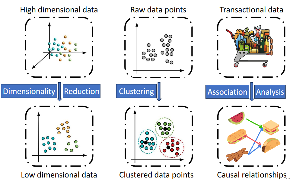
Figure: Unsupervised learning examples including dimensionality reduction, clustering and association analysis

• Semi-supervised Learning = learn from small set of labeled examples and large set of unlabeled data
• Reinforcement learning = learn from environment by interacting with it and receive rewards from performing actions

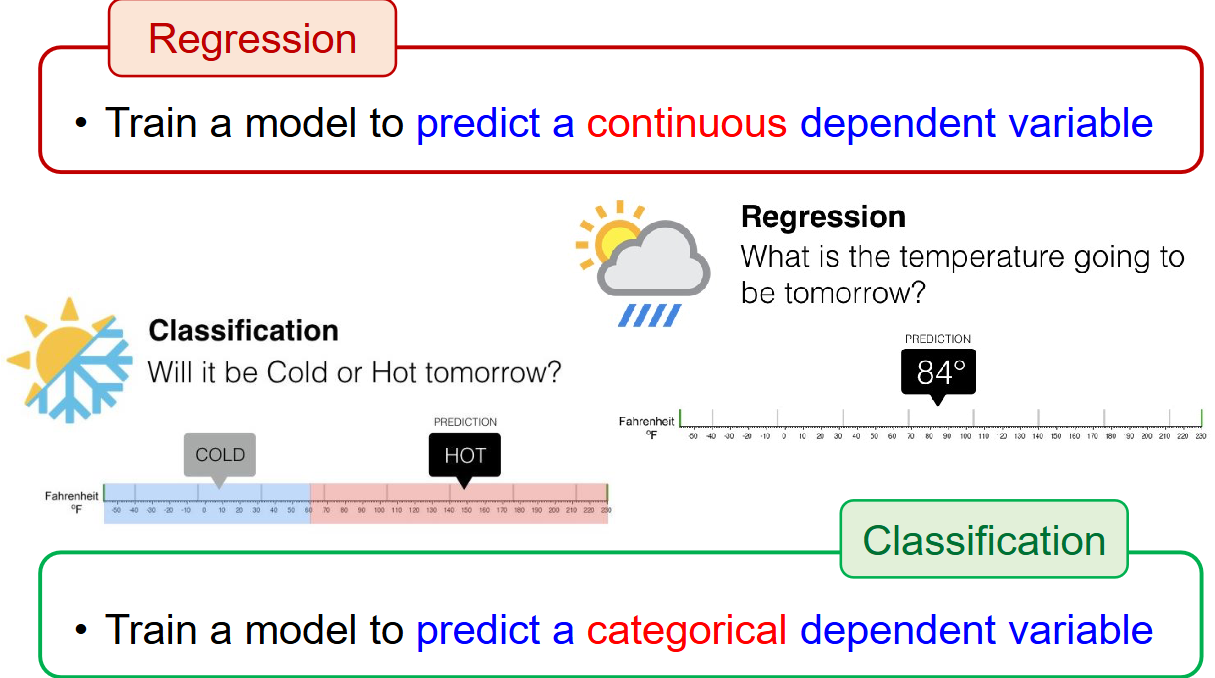
Figure: Comparison between supervised and unsupervised learning using example questions for temperature.

Then the real part is ID3 Decision Tree: a supervised learning method for classification. The core concept is Divide and conquer (Split data into smaller and smaller subsets using a single variable). We would want to split based on purity so that purity of each split increases. This means that the more we split, the better we can use certain traits to classify samples into the corresponding classes. The metric for this purity is Information Gain, which based on Entropy. The formula for entropy is $Entropy(H) = - \sum_{k} P(v_k) log_2 P(v_k)$ (random variable V with values $v_k$ having probability $P(v_k)$) and the formula for information gain is $H(S) - H(V)$ where $H(S)$ is entropy of the whole dataset.

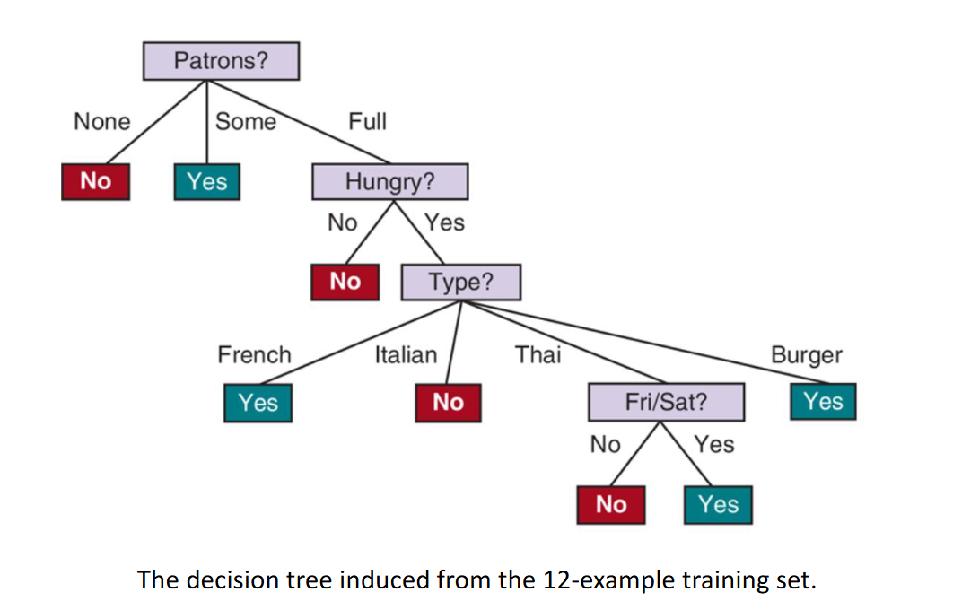
Figure: Full ID3 tree of an example dataset

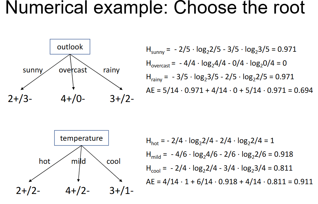
Figure: Example calculation of entropy for each value in variable and the entropy for the variable

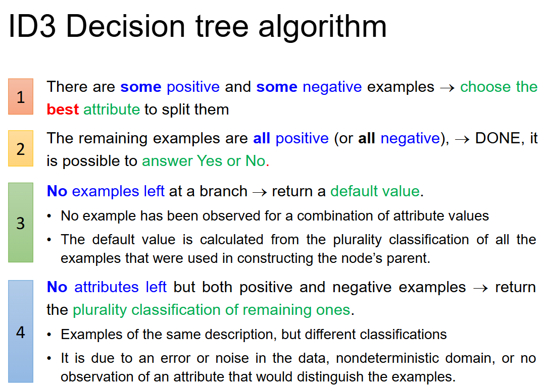
Figure: 4 edge cases illustrating ambiguous split choices.

Strategy to do this part quickly:

• Step 1: Calculate $H(S)$ for current tree (do not forget this step at each subtree)
• Step 2: For every variables, list all values together with number of instances in the value and the number of instances in each of the classes exists for that value.
• Step 3: For each value, we can use the number of instances in each of the classes exists for the value to calculate $H(V=v_k)$
• Step 4: Then we can use number of instances in the value to calculate $H(V)$
• Step 5: $IG(S, V) = H(S) - H(V)$
• Step 6: Branching and repeat step 1 (yes, at each subtree, we must start at calculate entropy of the dataset)

Some default value is:

• $n$ instances of $v_k$ and all of them belong to 1 class => $H(v_k)$ = 0
• $n$ instances of $v_k$ and all of them evenly distributed to 2 classes => $H(v_k)$ = 1

Deep Learning

A perceptron has a single neuron with adjustable synaptic weights and a hard limiter (with a defined threshold). Perceptron learning rule is simple: init -> activation -> weight update -> iterate. A fully connected feedforward network with at least three layers allows mapping inputs to specified target value.

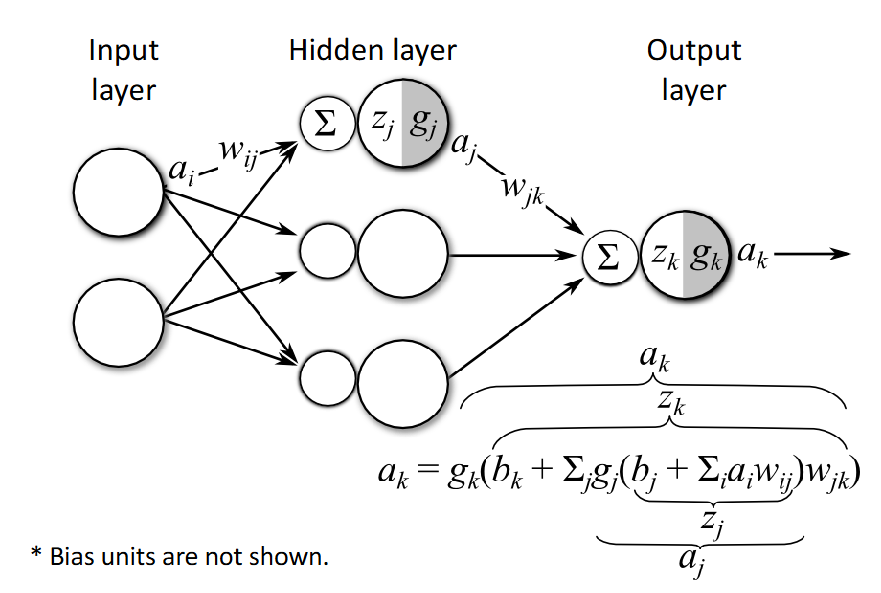
Figure: Multi-layer perceptron architecture with input, hidden, and output layers.

The weight update for output layer and hidden layers are different:

• Hidden layer (sigmoid): $w_{ij} \leftarrow w_{ij} - \eta \cdot \left(\sum_k \delta_k w_{jk}\right) \cdot y_j \cdot (1 - y_j) \cdot y_i$
• Output layer (sigmoid): $w_{jk} \leftarrow w_{jk} - \eta \cdot (y_k - y) \cdot y_k \cdot (1 - y_k) \cdot y_j$

The rule to remember is simple: to calculate the weight gradients at any layer $l$, we calculate the backpropagated error signal $\delta l$ that reaches that layer from the "afterward" layers, and weight it by the feed-forward signal at $l-1$ feeding into that layer.

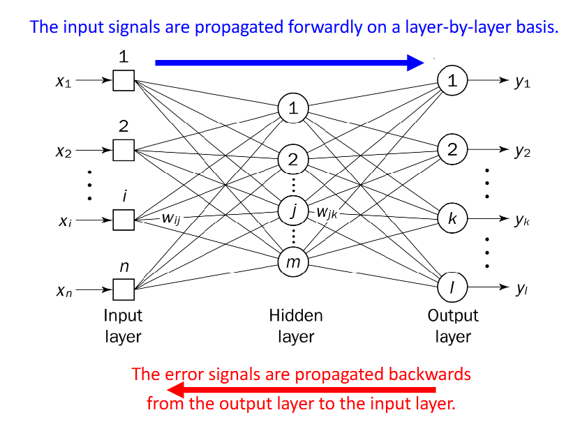
Figure: Backpropagation signal flow used to compute gradients and update weights.

And importantly, DO NOT FORGET ABOUT BIAS UPDATE RULE: $y_i = 1$ => IT MEANS NO WEIGHTING FOR THE ERROR TERM

The end?

Maybe.